Tutorial: Using R and Twitter to Analyse Consumer Sentiment
Content

This year I have been working with a Singapore Actuarial Society working party to introduce Singaporean actuaries to big data applications, and the new techniques and tools they need in order to keep up with this technology. The working group’s presentation at the 2015 General Insurance Seminar was well received, and people want more. So we are going to run some training tutorials, and want to extend our work.
One of those extensions is text mining. Inspired by a CAS paper by Roosevelt C. Mosly Jnr, I thought that I’d try to create a simple working example of twitter text mining, using R. I thought that I could just Google for an R script, make some minor changes, and run it. If only it were as simple as that…
I quickly ran into problems that none of the on-line blogs and documentation fully deal with:

• • Twitter changed its search API to require authorisation. That authorisation process is a bit time-consuming and even the most useful blogs got some minor but important details wrong.
  • CRAN has withdrawn its sentiment package, meaning that I couldn’t access the key R library that makes the example interesting.

After much experimentation, and with the help of some R experts, I finally created a working example. Here it goes, step by step:

STEP 1: Log on to https://apps.twitter.com/

Just use your normal Twitter account login. The screen should look like this:

STEP 2: Create a New Twitter Application

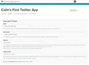
Click on the “Create New App” button, then you will be asked to fill in the following form:

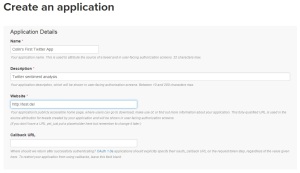
Choose your own application name, and your own application description. The website needs to be a valid URL. If you don’t have your own URL, then JULIANHI recommends that you use http://test.de/ , then scroll down the page.

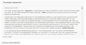
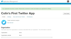
Click “Yes, I Agree” for the Developer Agreement, and then click the “Create your Twitter application” button. You will see something like this:

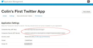
Go to the “Keys and Access Tokens” tab. Then look for the Consumer Key and the Consumer Secret. I have circled them in the image below. We will use these keys later in our R script, to authorise R to access the Twitter API.

Scroll down to the bottom of the page, where you will find the “Your Access Token” section.

Click on the button labelled “Create my access token”.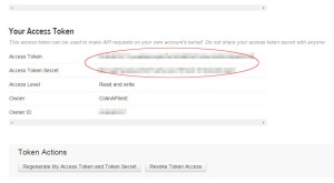

Look for the Access Token and Access Token Secret. We will use these in the next step, to authorise R to access the Twitter API.

STEP 3: Authorise R to Access Twitter

First we need to load the Twitter authorisation libraries. I like to use the pacman package to install and load my packages. The other packages we need are:

• • twitteR : which gives an R interface to the Twitter API
  • ROAuth : OAuth authentication to web servers
  • RCurl : http requests and processing the results returned by a web server

The R script is below. But first remember to replace each “xxx” with the respective token or secret you obtained from the Twitter app page.

# authorisation
if (!require('pacman')) install.packages('pacman')
pacman::p_load(twitteR, ROAuth, RCurl)

api_key = 'xxx'
api_secret = 'xxx'
access_token = 'xxx'
access_token_secret = 'xxx'

# Set SSL certs globally
options(RCurlOptions = list(cainfo = system.file('CurlSSL', 'cacert.pem', package = 'RCurl')))

# set up the URLs
reqURL = 'https://api.twitter.com/oauth/request_token'
accessURL = 'https://api.twitter.com/oauth/access_token'
authURL = 'https://api.twitter.com/oauth/authorize'

twitCred = OAuthFactory$new(consumerKey = api_key, consumerSecret = api_secret, requestURL = reqURL, accessURL = accessURL, authURL = authURL)

twitCred$handshake(cainfo = system.file('CurlSSL', 'cacert.pem', package = 'RCurl'))

After substituting your own token and secrets for “xxx”, run the script. It will open a web page in your browser. Note that on some systems R can’t open the browser automatically, so you will have to copy the URL from R, open your browser, then paste the link into your browser. If R gives you any error messages, then check that you have pasted the token and secret strings correctly, and ensure that you have the latest versions of the twitteR, ROAuth and RCurl libraries by reinstalling them using the install.packages command.

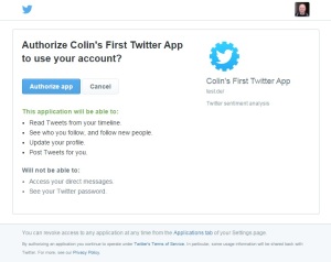
The web page will look something like this:

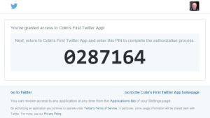
Click the “Authorise app” button, and you will be given a PIN (note that your PIN will be different to the one in my example).

Copy this PIN to the clipboard and then return to R, which is asking you to enter the PIN.

Paste in, or type, the PIN from the Twitter web page, then click enter. R is now authorised to run Twitter searches. You only need to do this once, but you do need to use your token strings and secret strings again in your R search scripts.

Go back to https://apps.twitter.com/ and go to the “Setup” tab for your application.

For the Callback URL enter http://127.0.0.1:1410 . This will allow us the option of an alternative authorisation method later.

STEP 4: Install the Sentiment Package

Since the sentiment package is no longer available on CRAN, we have to download the archived source code and install it via this RScript:

if (!require('pacman')) install.packages('pacman&')
pacman::p_load(devtools, installr)
install.Rtools()
install_url('http://cran.r-project.org/src/contrib/Archive/Rstem/Rstem_0.4-1.tar.gz')
install_url('http://cran.r-project.org/src/contrib/Archive/sentiment/sentiment_0.2.tar.gz')

Note that we only have to download and install the sentiment package once.

UPDATE: There’s a new package on CRAN for sentiment analysis, and I have written a tutorial about it.

STEP 5: Create A Script to Search Twitter

Finally we can create a script to search twitter. The first step is to set up the authorisation credentials for your script. This requires the following packages:

• twitteR : which gives an R interface to the Twitter API
• sentiment : classifies the emotions of text
• plyr : for splitting text
• ggplot2 : for plots of the categorised results
• wordcloud : creates word clouds of the results
• RColorBrewer :  colour schemes for the plots and wordcloud
• httpuv : required for the alternative web authorisation process
• RCurl : http requests and processing the results returned by a web server

if (!require('pacman')) install.packages('pacman')
pacman::p_load(twitteR, sentiment, plyr, ggplot2, wordcloud, RColorBrewer, httpuv, RCurl, base64enc)

options(RCurlOptions = list(cainfo = system.file('CurlSSL', 'cacert.pem', package = 'RCurl')))

api_key = 'xxx'
api_secret = 'xxx'
access_token = 'xxx'
access_token_secret = 'xxx'

setup_twitter_oauth(api_key,api_secret,access_token,access_token_secret)

Remember to replace the “xxx” strings with your token strings and secret strings.

Using the setup_twitter_oauth function with all four parameters avoids the case where R opens a web browser again. But I have found that it can be problematic to get this function to work on some computers. If you are having problems, then I suggest that you try the alternative call with just two parameters:

setup_twitter_oauth(api_key,api_secret)

This alternative way opens your browser and uses your login credentials from your current Twitter session.

Once authorisation is complete, we can run a search. For this example, I am doing a search on tweets mentioning a well-known brand: Starbucks. I am restricting the results to tweets written in English, and I am getting a sample of 10,000 tweets. It is also possible to give date range and geographic restrictions.

# harvest some tweets
some_tweets = searchTwitter('starbucks', n=10000, lang='en')

# get the text
some_txt = sapply(some_tweets, function(x) x$getText())

Please note that the Twitter search API does not return an exhaustive list of tweets that match your search criteria, as Twitter only makes available a sample of recent tweets. For a more comprehensive search, you will need to use the Twitter streaming API, creating a database of results and regularly updating them, or use an online service that can do this for you.

Now that we have tweet texts, we need to clean them up before doing any analysis. This involves removing content, such as punctuation, that has no emotional content, and removing any content that causes errors.

# remove retweet entities
some_txt = gsub('(RT|via)((?:\\b\\W*@\\w+)+)', '', some_txt)
# remove at people
some_txt = gsub('@\\w+', '', some_txt)
# remove punctuation
some_txt = gsub('[[:punct:]]', '', some_txt)
# remove numbers
some_txt = gsub('[[:digit:]]', '', some_txt)
# remove html links
some_txt = gsub('http\\w+', '', some_txt)
# remove unnecessary spaces
some_txt = gsub('[ \t]{2,}', '', some_txt)
some_txt = gsub('^\\s+|\\s+$', '', some_txt)

# define 'tolower error handling' function
try.error = function(x)
{
# create missing value
y = NA
# tryCatch error
try_error = tryCatch(tolower(x), error=function(e) e)
# if not an error
if (!inherits(try_error, 'error'))
y = tolower(x)
# result
return(y)
}
# lower case using try.error with sapply
some_txt = sapply(some_txt, try.error)

# remove NAs in some_txt
some_txt = some_txt[!is.na(some_txt)]
names(some_txt) = NULL

Now that we have clean text for analysis, we can do sentiment analysis. The classify_emotion function is from the sentiment package and “classifies the emotion (e.g. anger, disgust, fear, joy, sadness, surprise) of a set of texts using a naive Bayes classifier trained on Carlo Strapparava and Alessandro Valitutti’s emotions lexicon.”

# Perform Sentiment Analysis
# classify emotion
class_emo = classify_emotion(some_txt, algorithm='bayes', prior=1.0)
# get emotion best fit
emotion = class_emo[,7]
# substitute NA's by 'unknown'
emotion[is.na(emotion)] = 'unknown'

# classify polarity
class_pol = classify_polarity(some_txt, algorithm='bayes')
# get polarity best fit
polarity = class_pol[,4]
# Create data frame with the results and obtain some general statistics
# data frame with results
sent_df = data.frame(text=some_txt, emotion=emotion,
polarity=polarity, stringsAsFactors=FALSE)

# sort data frame
sent_df = within(sent_df,
emotion <- factor(emotion, levels=names(sort(table(emotion), decreasing=TRUE))))

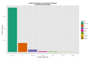
With the sentiment analysis done, we can start to look at the results. Let’s look at a histogram of the number of tweets with each emotion:

# Let’s do some plots of the obtained results
# plot distribution of emotions
ggplot(sent_df, aes(x=emotion)) +
geom_bar(aes(y=..count.., fill=emotion)) +
scale_fill_brewer(palette='Dark2') +
labs(x='emotion categories', y='number of tweets') +
ggtitle('Sentiment Analysis of Tweets about Starbucks\n(classification by emotion)') +
theme(plot.title = element_text(size=12, face='bold'))

Most of the tweets have unknown emotional content. But that sort of makes sense when there are tweets such as “With risky, diantri, and Rizky at Starbucks Coffee Big Mal”.

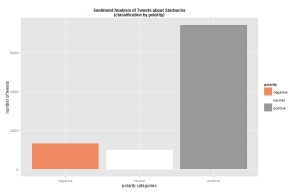
Let’s get a simpler plot, that just tells us whether the tweet is positive or negative.

# plot distribution of polarity
ggplot(sent_df, aes(x=polarity)) +
geom_bar(aes(y=..count.., fill=polarity)) +
scale_fill_brewer(palette='RdGy') +
labs(x='polarity categories', y='number of tweets') +
ggtitle('Sentiment Analysis of Tweets about Starbucks\n(classification by polarity)') +
theme(plot.title = element_text(size=12, face='bold'))

So it’s clear that most of the tweets are positive. That would explain why there are more than 21,000 Starbucks stores around the world!

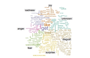
Finally, let’s look at the words in the tweets, and create a word cloud that uses the emotions of the words to determine their locations within the cloud.

# Separate the text by emotions and visualize the words with a comparison cloud
# separating text by emotion
emos = levels(factor(sent_df$emotion))
nemo = length(emos)
emo.docs = rep('', nemo)
for (i in 1:nemo)
{
tmp = some_txt[emotion == emos[i]]
emo.docs[i] = paste(tmp, collapse=' ')
}

# remove stopwords
emo.docs = removeWords(emo.docs, stopwords('english'))
# create corpus
corpus = Corpus(VectorSource(emo.docs))
tdm = TermDocumentMatrix(corpus)
tdm = as.matrix(tdm)
colnames(tdm) = emos

# comparison word cloud
comparison.cloud(tdm, colors = brewer.pal(nemo, 'Dark2'),
scale = c(3,.5), random.order = FALSE, title.size = 1.5)

Word clouds give a more intuitive feel for what people are tweeting. This can help you validate the categorical results you saw earlier.

And that’s it for this post! I hope that you can get Twitter sentiment analysis working on your computer too.

UPDATE: There’s a new package on CRAN for sentiment analysis, and I have written a tutorial about it.