In my last blog we had faded the coffee cup stains, but there was more work to be done. So far we had used adaptive thresholding and edge detection. Today we will use median filters and background removal.
A median filter is an image filter that replaces a pixel with the median value of the pixels surrounding it. In doing this, it smoothes the image, and the result is often thought of as the “background” of the image, since it tends to wipe away small features, but maintains broad features.
While the biOps package has a median filter implementation, it isn’t difficult to write a function to do that ourselves, and it can be quite instructive to see how a median filter works.
median_Filter = function(img, filterWidth)
{
 pad = floor(filterWidth / 2)
 padded = matrix(NA, nrow(img) + 2 * pad, ncol(img) + 2 * pad)
 padded[pad + seq_len(nrow(img)), pad + seq_len(ncol(img))] = img

 tab = NULL
 for (i in seq_len(filterWidth))
 {
 for (j in seq_len(filterWidth))
 {
 if (i == 1 && j == 1)
 {
 tab = img2vec(padded[i - 1 + seq_len(nrow(img)), j - 1 + seq_len(ncol(img))])
 } else {
 tab = cbind(tab, img2vec(padded[i - 1 + seq_len(nrow(img)), j - 1 + seq_len(ncol(img))]))
 }
 }
 }

 filtered = unlist(apply(tab, 1, function(x) median(x[!is.na(x)])))
 return (matrix(filtered, nrow(img), ncol(img)))
}

# libraries
if (!require("pacman")) install.packages("pacman")
pacman::p_load(png, raster)

# read in the coffee cup stain image
img = readPNG("C:\\Users\\Colin\\dropbox\\Kaggle\\Denoising Dirty Documents\\data\\train\\3.png")

# use the median filter and save the result
filtered = median_Filter(img, 17)
writePNG(filtered, "C:\\Users\\Colin\\dropbox\\Kaggle\\Denoising Dirty Documents\\data\\sample.png")
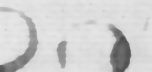
What we get after applying a median filter is something that looks like the background of the image. It contains the coffee cup stains and also the shade of the paper upon which the writing appears. With a filter width of 17, the writing has almost entirely faded away.
I didn’t choose that filter width of 17 randomly. It was the result of running models with several different filter widths and seeing which had the best predictive powers.
Median filters are not fast, especially once the filter width increases. This function runs with similar speed to that in the biOps package. I shall leave the task of writing a parallel processing version of the median filter function to the more impatient readers.
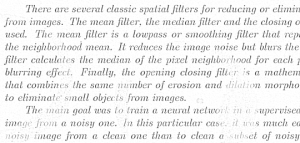
While we now have the background, what we really wanted was the foreground – the writing, without the coffee cup stains. The foreground is the difference between the original image and the background. But in this case we know that the writing is always darker than the background, so our foreground should only show pixels that are darker than the background. I have also rescaled the result to lie in the interval [0, 1]. Here is an R script to implement background removal.
# a function that uses median filter to get the background then finds the dark foreground
background_Removal = function(img)
{
 w = 5

 # the background is found via a median filter
 background = median_Filter(img, w)

 # the foreground is darker than the background
 foreground = img - background
 foreground[foreground > 0] = 0
 m1 = min(foreground)
 m2 = max(foreground)
 foreground = (foreground - m1) / (m2 - m1)

 return (matrix(foreground, nrow(img), ncol(img)))
}

# run the background removal function and save the result
foreground = background_Removal(img)
writePNG(foreground, "C:\\Users\\Colin\\dropbox\\Kaggle\\Denoising Dirty Documents\\data\\sample.png")
While it’s not perfect, the resulting filtered image has done a reasonably good job of separating the writing from the background. It is reasonable to expect that it will be a useful predictor in our model.
This time a filter width of 5 was chosen purely for the purpose of speed. You could have used a grid search to find the “best” filter width parameter.
# read in the coffee cup stain image
img = readPNG("C:\\Users\\Colin\\dropbox\\Kaggle\\Denoising Dirty Documents\\data\\train\\3.png")
imgClean = readPNG("C:\\Users\\Colin\\dropbox\\Kaggle\\Denoising Dirty Documents\\data\\train_cleaned\\3.png")

bestRMSE = 1
bestWidth = 5

widths = c(3, 5, 7, 9, 11, 13, 15, 17, 19, 21, 23, 25)

for (w in widths)
{
 # the background is found via a median filter
 background = median_Filter(img, w)

 # the foreground is darker than the background
 foreground = img - background
 foreground[foreground > 0] = 0
 m1 = min(foreground)
 m2 = max(foreground)
 foreground = (foreground - m1) / (m2 - m1)

 # score the result
 rmse = sqrt(mean( (foreground - imgClean) ^ 2 ))
 if (rmse < bestRMSE)
 {
 bestRMSE = rmse
 bestWidth = w
 print(c(bestWidth, rmse))
 }
}
In the past few blogs I have used the GBM package to create a predictive model. But as we have added more predictors or features, it has started to take a long time to fit the model and to calculate the predictions. So today I’m switching to the xgboost package because the top Kagglers are using it (Owen Zhang, Kaggle’s top ranked competitor says “when in doubt use xgboost“), and because it runs much faster than GBM. I’d never used xgboost until this week, and I must say that I’m quite impressed with its speed.
Here is an R script that fits an xgboost model, using all of the features that we have come up with over the 5 blogs to date.
# libraries
if (!require("pacman")) install.packages("pacman")
pacman::p_load(png, raster, data.table, gbm, foreach, doSNOW, biOps, xgboost, Ckmeans.1d.dp)

if (!require("EBImage"))
{
 source("http://bioconductor.org/biocLite.R")
 biocLite("EBImage")
}

# a function to do k-means thresholding
kmeansThreshold = function(img)
{
 # fit 3 clusters
 v = img2vec(img)
 km.mod = kmeans(v, 3)
 # allow for the random ordering of the clusters
 oc = order(km.mod$centers)
 # the higher threshold is the halfway point between the top of the middle cluster and the bottom of the highest cluster
 hiThresh = 0.5 * (max(v[km.mod$cluster == oc[2]]) + min(v[km.mod$cluster == oc[3]]))

 # using upper threshold
 imgHi = v
 imgHi[imgHi <= hiThresh] = 0 imgHi[imgHi > hiThresh] = 1

 return (imgHi)
}

# a function that applies adaptive thresholding
adaptiveThresholding = function(img)
{
 img.eb <- Image(t(img))
 img.thresholded.3 = thresh(img.eb, 3, 3)
 img.thresholded.5 = thresh(img.eb, 5, 5)
 img.thresholded.7 = thresh(img.eb, 7, 7)
 img.thresholded.9 = thresh(img.eb, 9, 9)
 img.thresholded.11 = thresh(img.eb, 11, 11)
 img.kmThresh = kmeansThreshold(img)

 # combine the adaptive thresholding
 ttt.1 = cbind(img2vec(Image2Mat(img.thresholded.3)), img2vec(Image2Mat(img.thresholded.5)), img2vec(Image2Mat(img.thresholded.7)), img2vec(Image2Mat(img.thresholded.9)), img2vec(Image2Mat(img.thresholded.11)), img2vec(kmeansThreshold(img)))
 ttt.2 = apply(ttt.1, 1, max)
 ttt.3 = matrix(ttt.2, nrow(img), ncol(img))
 return (ttt.3)
}

# a function to turn a matrix image into a vector
img2vec = function(img)
{
 return (matrix(img, nrow(img) * ncol(img), 1))
}

# a function to convert an Image into a matrix
Image2Mat = function(Img)
{
 m1 = t(matrix(Img, nrow(Img), ncol(Img)))
 return(m1)
}

# a function to do canny edge detector
cannyEdges = function(img)
{
 img.biOps = imagedata(img * 255)
 img.canny = imgCanny(img.biOps, 0.7)
 return (matrix(img.canny / 255, nrow(img), ncol(img)))
}

# a function combining canny edge detector with morphology
cannyDilated1 = function(img)
{
 img.biOps = imagedata(img * 255)
 img.canny = imgCanny(img.biOps, 0.7)
 # do some morphology on the edges to fill the gaps between them
 mat <- matrix (0, 3, 3)
 mask <- imagedata (mat, "grey", 3, 3)
 img.dilation = imgBinaryDilation(img.canny, mask)
 img.erosion = imgBinaryErosion(img.dilation, mask)
 return(matrix(img.erosion / 255, nrow(img), ncol(img)))
}

# a function combining canny edge detector with morphology
cannyDilated2 = function(img)
{
 img.biOps = imagedata(img * 255)
 img.canny = imgCanny(img.biOps, 0.7)
 # do some morphology on the edges to fill the gaps between them
 mat <- matrix (0, 3, 3)
 mask <- imagedata (mat, "grey", 3, 3) img.dilation = imgBinaryDilation(img.canny, mask) img.erosion = imgBinaryErosion(img.dilation, mask) img.erosion.2 = imgBinaryErosion(img.erosion, mask) img.dilation.2 = imgBinaryDilation(img.erosion.2, mask) return(matrix(img.dilation.2 / 255, nrow(img), ncol(img))) } # a function to do a median filter median_Filter = function(img, filterWidth) { pad = floor(filterWidth / 2) padded = matrix(NA, nrow(img) + 2 * pad, ncol(img) + 2 * pad) padded[pad + seq_len(nrow(img)), pad + seq_len(ncol(img))] = img tab = NULL for (i in seq_len(filterWidth)) { for (j in seq_len(filterWidth)) { if (i == 1 && j == 1) { tab = img2vec(padded[i - 1 + seq_len(nrow(img)), j - 1 + seq_len(ncol(img))]) } else { tab = cbind(tab, img2vec(padded[i - 1 + seq_len(nrow(img)), j - 1 + seq_len(ncol(img))])) } } } filtered = unlist(apply(tab, 1, function(x) median(x[!is.na(x)]))) return (matrix(filtered, nrow(img), ncol(img))) } # a function that uses median filter to get the background then finds the dark foreground background_Removal = function(img) { w = 5 # the background is found via a median filter background = median_Filter(img, w) # the foreground is darker than the background foreground = img - background foreground[foreground > 0] = 0
 m1 = min(foreground)
 m2 = max(foreground)
 foreground = (foreground - m1) / (m2 - m1)

 return (matrix(foreground, nrow(img), ncol(img)))
}

dirtyFolder = "C:\\Users\\Colin\\dropbox\\Kaggle\\Denoising Dirty Documents\\data\\train"
cleanFolder = "C:\\Users\\Colin\\dropbox\\Kaggle\\Denoising Dirty Documents\\data\\train_cleaned"
outFolder = "C:\\Users\\Colin\\dropbox\\Kaggle\\Denoising Dirty Documents\\data\\train_predicted"

outPath = file.path(outFolder, "trainingdata_blog5.csv")
filenames = list.files(dirtyFolder)
for (f in filenames)
{
 print(f)
 imgX = readPNG(file.path(dirtyFolder, f))
 imgY = readPNG(file.path(cleanFolder, f))

 # turn the images into vectors
 x = matrix(imgX, nrow(imgX) * ncol(imgX), 1)
 y = matrix(imgY, nrow(imgY) * ncol(imgY), 1)

 # threshold the image
 x2 = kmeansThreshold(imgX)

 # adaptive thresholding
 x3 = img2vec(adaptiveThresholding(imgX))

 # canny edge detector and related features
 x4 = img2vec(cannyEdges(imgX))
 x5 = img2vec(cannyDilated1(imgX))
 x6 = img2vec(cannyDilated2(imgX))

 # median filter and related features
 x7 = img2vec(median_Filter(imgX, 17))
 x8 = img2vec(background_Removal(imgX))

 dat = data.table(cbind(y, x, x2, x3, x4, x5, x6, x7, x8))
 setnames(dat,c("y", "raw", "thresholded", "adaptive", "canny", "cannyDilated1", "cannyDilated2", "median17", "backgroundRemoval"))
 write.table(dat, file=outPath, append=(f != filenames[1]), sep=",", row.names=FALSE, col.names=(f == filenames[1]), quote=FALSE)
}

# read in the full data table
dat = read.csv(outPath)

# fit an xgboost model to a subset of the data
set.seed(1)
rows = sample(nrow(dat), 2000000)
dat[is.na(dat)] = 0
dtrain <- xgb.DMatrix(as.matrix(dat[rows,-1]), label = as.matrix(dat[rows,1]))
# do cross validation first
xgb.tab = xgb.cv(data = dtrain, nthread = 8, eval_metric = "rmse", nrounds = 10000, early.stop.round = 50, nfold = 5, print.every.n = 10)
# what is the best number of rounds?
min.error.idx = which.min(xgb.tab[, test.rmse.mean])
# now fit an xgboost model
xgb.mod = xgboost(data = dtrain, nthread = 8, eval_metric = "rmse", nrounds = min.error.idx, print.every.n = 10)

# get the predictions
dtrainFull <- xgb.DMatrix(as.matrix(dat[,-1]), label = as.matrix(dat[,1]))
yHat = predict(xgb.mod, newdata=dtrainFull)
# what score do we get on the training data?
rmse = sqrt(mean( (yHat - dat$y) ^ 2 ))
print(rmse) # 2.4% vs 4.1%

# get the trained model
model = xgb.dump(xgb.mod, with.stats=TRUE)
# get the feature real names
names = names(dat)[-1]
# compute feature importance matrix
importance_matrix = xgb.importance(names, model=xgb.mod)
# plot the variable importance
gp = xgb.plot.importance(importance_matrix)
print(gp)


# show the predicted result for a sample image
img = readPNG("C:\\Users\\Colin\\dropbox\\Kaggle\\Denoising Dirty Documents\\data\\train\\3.png")
x = data.table(matrix(img, nrow(img) * ncol(img), 1), kmeansThreshold(img), img2vec(adaptiveThresholding(img)), img2vec(cannyEdges(img)),
 img2vec(cannyDilated1(img)), img2vec(cannyDilated2(img)),img2vec(median_Filter(img, 17)), img2vec(background_Removal(img)) )
setnames(x, c("raw", "thresholded", "adaptive", "canny", "cannyDilated1", "cannyDilated2", "median17", "backgroundRemoval"))
yHatImg = predict(xgb.mod, newdata=as.matrix(x))
yHatImg[yHatImg < 0] = 0 yHatImg[yHatImg > 1] = 1
imgOut = matrix(yHatImg, nrow(img), ncol(img))
writePNG(imgOut, "C:\\Users\\Colin\\dropbox\\Kaggle\\Denoising Dirty Documents\\data\\sample.png")
plot(raster(imgOut))
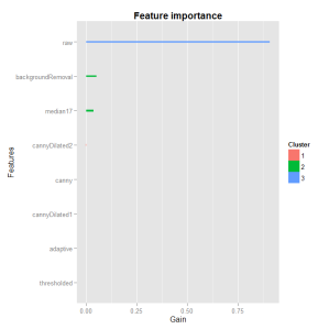
Both the background removal and the median filter features are important, with even higher importance scores than last blog’s canny edge detector features.
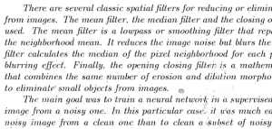
The coffee cup stain has been mostly removed, especially the speckles that we saw after applying the model in the last blog.
The result represents an improvement in RMSE score on the training data from 4.1% in the last blog to 2.4% in this blog. In the next blog we will further improve on this score.


Great stuff Colin! I’ve been looking for sliding window code so I’m glad you chose to implement the median filter from scratch instead of using a library.
In one of my submissions, I used a gaussian filter instead which helped my score a bit. I haven’t compared the median filter to the gaussian filter yet but I was wondering if there should be some particular preference here when it comes to the image data we’re working with?
Cheers.
LikeLiked by 1 person
Hi Bobby,
Gaussian filters are much faster because they can use a convolutional filter, and our CPUs and GPUs are optimised for convolution operations. A median filter is good for finding a “typical” pixel brightness, because it ignores extremes. A Gaussian filter reacts more to one or two very different pixels, and is intended for smoothing rather than finding the background. A difference-of-gaussians (DoG) is good for finding features with a particular width.
Colin
LikeLike
Ah ok, thanks for the explanation.
I was also wondering if we’re just using the backgroundRemoval feature to train the xgboost model? The reason I ask is because that’s what the following code looks like its doing:
dtrain <- xgb.DMatrix(as.matrix(dat[rows,-1]), label = as.matrix(dat[rows,1]))
If that is the case, why not use all the features?
LikeLike
Bobby,
We are using all of the features. That line of code just formats the data into a DMatrix, splitting the target (the first column) from the predictors, which is what xgboost wants as input.
You can tell that xgboost is using all of the features because the variable importance shows that they are being used.
Colin
LikeLike
Pingback: Denoising Dirty Documents: Part 6 | Keeping Up With The Latest Techniques
Pingback: Denoising Dirty Documents: Part 7 | Keeping Up With The Latest Techniques
biOps package is removed from R-3.2.2. Any alternative package from some other source. biOps is not installing from any outside source
LikeLike
Hi Ramit,
Have you had any success installing biOps from the CRAN archive?
LikeLike
Pingback: Image Processing + Machine Learning in R: Denoising Dirty Documents Tutorial Series | No Free Hunch
which version 0f R you have used?
LikeLike
Hi Sparsh. Sorry I can’t remember which version of R I was using when I wrote this. But the R scripts should work on any recent version of R. Colin
LikeLike
Pingback: learn Data Science by doing | Egyptian AI & Big Data Geeks Offical Blog