Keeping Up With The Latest Techniques

~ brief insights

Keeping Up With The Latest Techniques

Tag Archives: Text Mining

Tutorial: Sentiment Analysis of Airlines Using the syuzhet Package and Twitter

30 Sunday Apr 2017

Posted by Colin Priest in R, Sentiment Analysis, Social Media, Text Mining, Twitter

≈ 32 Comments

Tags

R, Sentiment Analysis, Text Mining, Twitter

In my last job, I was a frequent flyer. Each week I flew between 2 or 3 countries, briefly returning for 24 hours on the weekend to get a change of clothes. My favourite airlines were Cathay Pacific, Emirates and Singapore Air. Now, unless you have been living in a cave, you’d be well aware of the recent news story of how United Airlines removed David Dao from an aircraft. I wondered how that incident had affected United’s brand value, and being a data scientist I decided to do sentiment analysis of United versus my favourite airlines.

Way back on 4th July 2015, almost two years ago, I wrote a blog entitled Tutorial: Using R and Twitter to Analyse Consumer Sentiment. Even though that blog post is one of my earliest, it continues to be the most popular, attracting just as many readers per day as when I first wrote it.

Since the sentiment package, upon which that blog was based, is no longer supported by CRAN, and many readers have problems with the manual and technical process of installing an obsolete package from an archive, I have written a new blog using a different, live CRAN package. The syuzhet package was published only several weeks ago, and offers a range of different sentiment analysis models. So I’ve started to try it out.

I have collected tweets for 4 airlines:

  1. Cathay Pacific
  2. Emirates
  3. Singapore Air
  4. United Airlines

The tweet data starts at 01-Jan-2015 and go up to mid-April 2017.

Step 1: Load the tweets and load the relevant packages

library(foreign)
library(syuzhet)
library(lubridate)
library(plyr)
library(ggplot2)
library(tm)
library(wordcloud)

# get the data for the tweets
dataURL = 'https://s3-ap-southeast-1.amazonaws.com/colinpriest/tweets.zip'
if (! file.exists('tweets.zip')) download.file(dataURL, 'tweets.zip')
if (! file.exists('tweets.dbf')) unzip('tweets.zip')
tweets = read.dbf('tweets.dbf', as.is = TRUE)


I’ve stored the tweets in a dbf file and zipped it. The zip file is 68MB in size, and the dbf file is 353MB. The code shown above downloads the zip file, extracts the dbf and then reads the dbf file into a data.frame.

Step 2: Do Sentiment Scoring using the syuzhet package


# function to get various sentiment scores, using the syuzhet package
scoreSentiment = function(tab)
{
 tab$syuzhet = get_sentiment(tab$Text, method="syuzhet")
 tab$bing = get_sentiment(tab$Text, method="bing")
 tab$afinn = get_sentiment(tab$Text, method="afinn")
 tab$nrc = get_sentiment(tab$Text, method="nrc")
 emotions = get_nrc_sentiment(tab$Text)
 n = names(emotions)
 for (nn in n) tab[, nn] = emotions[nn]
 return(tab)
}

# get the sentiment scores for the tweets
tweets = scoreSentiment(tweets)
tweets = tweets[tweets$TimeStamp < as.Date('19-04-2017', format = '%d-%m-%Y'),]

The syuzhet package offers a few different algorithms, each taking a different approach to sentiment scoring. It also does emotion scoring based upon the nrc algorithm. The code above calculates scores using the syuzhet, bing, afinn and nrc algorithms, adding columns with the scores from each algorithm.

Step 3: Visualise the Sentiment Scores


# function to find the week in which a date occurs
round_weeks <- function(x)
{
require(data.table)
dt = data.table(i = 1:length(x), day = x, weekday = weekdays(x))
offset = data.table(weekday = c('Sunday', 'Monday', 'Tuesday', 'Wednesday',
'Thursday', 'Friday', 'Saturday'),
offset = -(0:6))
dt = merge(dt, offset, by="weekday")
dt[ , day_adj := day + offset]
setkey(dt, i)
return(dt[ , day_adj])
}
# get daily summaries of the results
daily = ddply(tweets, ~ Airline + TimeStamp, summarize, num_tweets = length(positive), ave_sentiment = mean(bing),
 ave_negative = mean(negative), ave_positive = mean(positive), ave_anger = mean(anger))

# plot the daily sentiment
ggplot(daily, aes(x=TimeStamp, y=ave_sentiment, colour=Airline)) + geom_line() +
 ggtitle("Airline Sentiment") + xlab("Date") + ylab("Sentiment") + scale_x_date(date_labels = '%d-%b-%y')

# get weekly summaries of the results
weekly = ddply(tweets, ~ Airline + week, summarize, num_tweets = length(positive), ave_sentiment = mean(bing),
 ave_negative = mean(negative), ave_positive = mean(positive), ave_anger = mean(anger))

# plot the weekly sentiment
ggplot(weekly, aes(x=week, y=ave_sentiment, colour=Airline)) + geom_line() +
 ggtitle("Airline Sentiment") + xlab("Date") + ylab("Sentiment") + scale_x_date(date_labels = '%d-%b-%y')

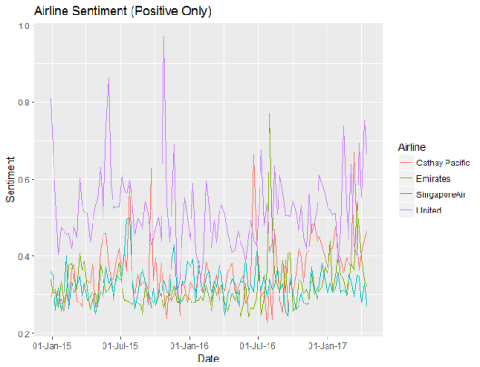
The code above summarises the sentiment for each airline across time. The first plot shows the daily sentiment values for each airline:

20170429 plot 01 daily sentiment

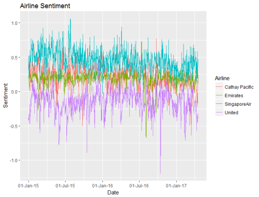
Based upon the bing sentiment algorithm, United has the poorest sentiment, and Singapore has the best sentiment. United usually has negative sentiment. Daily to day random fluctuations in sentiment make this a cluttered graph, so I decided to summarise the sentiment weekly instead of daily:

20170429 plot 02 weekly sentiment

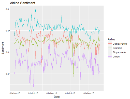
Now it’s easier to see the differences in sentiment between the four airlines. While Emirates and Cathay Pacific have similar levels of sentiment, the values for Emirates are more stable. This, however, may be due to the sheer volume of tweets about Emirates versus the smaller number of tweets about Cathay Pacific.

20170429 plot 03 positive sentiment

Step 4: Compare the Sentiment Algorithms

The sentiment scores above use the bing algorithm, but we should check whether the different algorithms produce different results.


# compare the sentiment for across the algorithms
algorithms = tweets[rep(1, nrow(tweets) * 4), c("week", "syuzhet", "Airline", "Airline")]
names(algorithms) = c("TimeStamp", "Sentiment", "Algorithm", "Airline")
algorithms$Algorithm = "syuzhet"
algorithms[seq_len(nrow(tweets)), c("TimeStamp", "Sentiment", "Airline")] = tweets[,c("TimeStamp", "syuzhet", "Airline")]
algorithms[nrow(tweets) + seq_len(nrow(tweets)), c("TimeStamp", "Sentiment", "Airline")] = tweets[,c("TimeStamp", "bing", "Airline")]
algorithms$Algorithm[nrow(tweets) + seq_len(nrow(tweets))] = "bing"
algorithms[2 * nrow(tweets) + seq_len(nrow(tweets)), c("TimeStamp", "Sentiment", "Airline")] = tweets[,c("TimeStamp", "afinn", "Airline")]
algorithms$Algorithm[2 * nrow(tweets) + seq_len(nrow(tweets))] = "afinn"
algorithms[3 * nrow(tweets) + seq_len(nrow(tweets)), c("TimeStamp", "Sentiment", "Airline")] = tweets[,c("TimeStamp", "nrc", "Airline")]
algorithms$Algorithm[3 * nrow(tweets) + seq_len(nrow(tweets))] = "nrc"

# get the algorithm averages for each airline
averages = ddply(algorithms, ~ Airline + Algorithm, summarize, ave_sentiment = mean(Sentiment))
averages$ranking = 1
for (alg in c("syuzhet", "bing", "afinn", "nrc")) averages$ranking[averages$Algorithm == alg] = 5 - rank(averages$ave_sentiment[averages$Algorithm == alg])
averages = averages[order(averages$Airline, averages$Algorithm), ]

The code above was a bit clumsy – I probably should have used reshape.

20170429 plot 08 sentiment algorithm comparisons

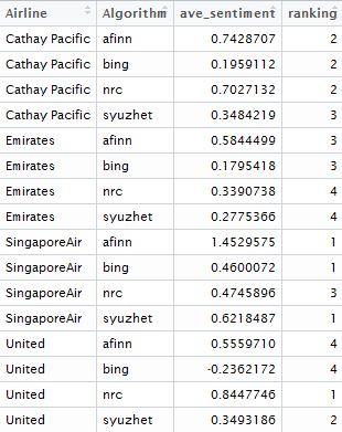
The different algorithms give similar rankings between the airlines with one big exception: the nrc algorithm is surprisingly positive about United and unusually negative about Singapore Air compared to the other algorithms. This goes to show that sentiment analysis isn’t just a plug and play technique and also means that a warning should be applied to the emotion analysis shown in Step 5 below, as it is based upon the nrc algorithm!

Step 5: Emotion Analysis

Noting the warning, from the previous section, let’s compare the emotions between the airlines and between tweets, using the nrc algorithm.


ggplot(weekly, aes(x=week, y=ave_negative, colour=Airline)) + geom_line() +
ggtitle("Airline Sentiment (Positive Only)") + xlab("Date") + ylab("Sentiment") + scale_x_date(date_labels = '%d-%b-%y')

ggplot(weekly, aes(x=week, y=ave_positive, colour=Airline)) + geom_line() +
ggtitle("Airline Sentiment (Negative Only)") + xlab("Date") + ylab("Sentiment") + scale_x_date(date_labels = '%d-%b-%y')

ggplot(weekly, aes(x=week, y=ave_anger, colour=Airline)) + geom_line() +
ggtitle("Airline Sentiment (Anger Only)") + xlab("Date") + ylab("Sentiment") + scale_x_date(date_labels = '%d-%b-%y')

# function to make the text suitable for analysis
clean.text = function(x)
{
# tolower
x = tolower(x)
# remove rt
x = gsub("rt", "", x)
# remove at
x = gsub("@\\w+", "", x)
# remove punctuation
x = gsub("[[:punct:]]", "", x)
# remove numbers
x = gsub("[[:digit:]]", "", x)
# remove links http
x = gsub("http\\w+", "", x)
# remove tabs
x = gsub("[ |\t]{2,}", "", x)
# remove blank spaces at the beginning
x = gsub("^ ", "", x)
# remove blank spaces at the end
x = gsub(" $", "", x)
return(x)
}

# emotion analysis: anger, anticipation, disgust, fear, joy, sadness, surprise, trust
# put everything in a single vector
all = c(
paste(tweets$Text[tweets$anger > 0], collapse=" "),
paste(tweets$Text[tweets$anticipation > 0], collapse=" "),
paste(tweets$Text[tweets$disgust > 0], collapse=" "),
paste(tweets$Text[tweets$fear > 0], collapse=" "),
paste(tweets$Text[tweets$joy > 0], collapse=" "),
paste(tweets$Text[tweets$sadness > 0], collapse=" "),
paste(tweets$Text[tweets$surprise > 0], collapse=" "),
paste(tweets$Text[tweets$trust > 0], collapse=" ")
)
# clean the text
all = clean.text(all)
# remove stop-words
# adding extra domain specific stop words
all = removeWords(all, c(stopwords("english"), 'singapore', 'singaporeair',
'emirates', 'united', 'airlines', 'unitedairlines',
'cathay', 'pacific', 'cathaypacific', 'airline',
'airlinesunited', 'emiratesemirates', 'pacifics'))
#
# create corpus
corpus = Corpus(VectorSource(all))
#
# create term-document matrix
tdm = TermDocumentMatrix(corpus)
#
# convert as matrix
tdm = as.matrix(tdm)
#
# add column names
colnames(tdm) = c('anger', 'anticipation', 'disgust', 'fear', 'joy', 'sadness', 'surprise', 'trust')
#
# Plot comparison wordcloud
layout(matrix(c(1, 2), nrow=2), heights=c(1, 4))
par(mar=rep(0, 4))
plot.new()
text(x=0.5, y=0.5, 'Emotion Comparison Word Cloud')
comparison.cloud(tdm, random.order=FALSE,
colors = c("#00B2FF", "red", "#FF0099", "#6600CC", "green", "orange", "blue", "brown"),
title.size=1.5, max.words=250)

&nbsp;

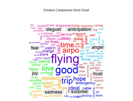
The code above plots the emotions across time for each airline.

20170429 plot 05 anger
20170429 plot 03 positive sentiment
20170429 plot 04 negative sentiment

United Airlines attracts more angry tweets, and this has spiked in April 2017 following the David Dao incident. But United Airlines also attracts more positive tweets than the other airlines. This might explain the ranking differences between the algorithms – maybe the algorithms weight positive tweets differently to negative tweets.

Then the code creates a comparison word cloud, to show the different words in airline tweets that are associated with each emotion.

20170429 plot 09 emotions

Step 6: Compare the Different Tweeting Behaviour of Different Twitter Users

Are some users more positive than others? Is this user behaviour different between the airlines? Do people who tweet more have a different sentiment to those who tweet about airlines less frequently? Are particular users dragging the average up or down? To answer these questions, I have tracked the 100 users who tweeted the most about these airlines.


# get the user summaries of the results
users = ddply(tweets, ~ Airline + UserName, summarize, num_tweets = length(positive), ave_sentiment = mean(bing),
ave_negative = mean(negative), ave_positive = mean(positive), ave_anger = mean(anger))
sizeSentiment = ddply(users, ~ num_tweets, summarize, ave_sentiment = mean(ave_sentiment),
ave_negative = mean(ave_negative), ave_positive = mean(ave_positive), ave_anger = mean(ave_anger))
sizeSentiment$num_tweets = as.numeric(sizeSentiment$num_tweets)

# plot users positive versus negative with bubble plot
cutoff = sort(users$num_tweets, decreasing = TRUE)[100]
ggplot(users[users$num_tweets > cutoff,], aes(x = ave_positive, y = ave_negative, size = num_tweets, fill = Airline)) +
geom_point(shape = 21) +
ggtitle("100 Most Prolific Tweeters About Airlines") +
labs(x = "Positive Sentiment", y = "Negative Sentiment")
#
ggplot(sizeSentiment, aes(x = num_tweets, y = ave_sentiment)) + geom_point() + stat_smooth(method = "loess", size = 1, span = 0.35) +
ggtitle("Number of Tweets versus Sentiment") + scale_x_log10() +
labs(x = "Positive Sentiment", y = "Negative Sentiment")

Firstly let’s look at the behaviour of individual users:

20170429 plot 06 top 100 tweeters

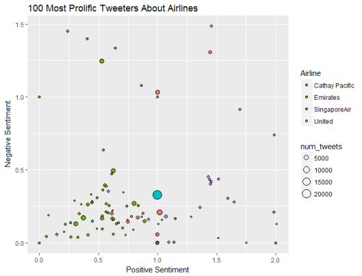
Top user sentiment is quite different by airline. Emirates has a number of frequent tweeters who are unemotional, who on average post neither positive nor negative sentiment. United Airlines attracts more emotional posts. Singapore Air and Cathay Pacific have big users that post a lot of tweets about them.

20170429 plot 07 sentiment versus tweet count

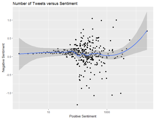
However, on average bigger frequent tweeters post a similar balance of positive and negative content to smaller users who tweet infrequently.

Step 7: Compare The Words Used to Describe Each Airline

In order to explain the differences in sentiment, we can create a word cloud that contrasts the words used in posts about each airline.


# Join texts in a vector for each company
txt1 = paste(tweets$Text[tweets$Airline == 'United'], collapse=" ")
txt2 = paste(tweets$Text[tweets$Airline == 'SingaporeAir'], collapse=" ")
txt3 = paste(tweets$Text[tweets$Airline == 'Emirates'], collapse=" ")
txt4 = paste(tweets$Text[tweets$Airline == 'Cathay Pacific'], collapse=" ")
#
# put everything in a single vector
all = c(clean.text(txt1), clean.text(txt2), clean.text(txt3), clean.text(txt4))
#
# remove stop-words
# adding extra domain specific stop words
all = removeWords(all, c(stopwords("english"), 'singapore', 'singaporeair',
'emirates', 'united', 'airlines', 'unitedairlines',
'cathay', 'pacific', 'cathaypacific', 'airline',
'airlinesunited', 'emiratesemirates', 'pacifics'))
#
# create corpus
corpus = Corpus(VectorSource(all))
#
# create term-document matrix
tdm = TermDocumentMatrix(corpus)
#
# convert as matrix
tdm = as.matrix(tdm)
#
# add column names
colnames(tdm) = c('United', 'Singapore Air', 'Emirates', 'Cathay Pacific')
#
# Plot comparison wordcloud
layout(matrix(c(1, 2), nrow=2), heights=c(1, 4))
par(mar=rep(0, 4))
plot.new()
text(x=0.5, y=0.5, 'Word Comparison by Airline')
comparison.cloud(tdm, random.order=FALSE,
colors = c("#00B2FF", "red", "#FF0099", "#6600CC"),
title.size=1.5, max.words=250)
#
# Plot commonality cloud
layout(matrix(c(1, 2), nrow=2), heights=c(1, 4))
par(mar=rep(0, 4))
plot.new()
text(x=0.5, y=0.5, 'Word Commonality by Airline')
commonality.cloud(tdm, random.order=FALSE,
colors = brewer.pal(8, "Dark2"),
title.size=1.5, max.words=250)

The code above is quite similar to that in the previous step, except that this time we are comparing airlines instead of emotions.

20170429 plot 10 airline word contrast
20170429 plot 11 airline word commonality

Emirates includes “aniston”, presumably in reference to the marketing campaign involving Jennifer Aniston, while United includes “CEO” due to a number of news stories about United CEO’s including a resignation and a heart transplant.


Share this:

  • Twitter
  • Facebook

Like this:

Like Loading...

Tutorial: Using R and Twitter to Analyse Consumer Sentiment

04 Saturday Jul 2015

Posted by Colin Priest in R, Text Mining, Twitter

≈ 145 Comments

Tags

R, Text Mining, Twitter

Tutorial: Using R and Twitter to Analyse Consumer Sentiment
Content

This year I have been working with a Singapore Actuarial Society working party to introduce Singaporean actuaries to big data applications, and the new techniques and tools they need in order to keep up with this technology. The working group’s presentation at the 2015 General Insurance Seminar was well received, and people want more. So we are going to run some training tutorials, and want to extend our work.
One of those extensions is text mining. Inspired by a CAS paper by Roosevelt C. Mosly Jnr, I thought that I’d try to create a simple working example of twitter text mining, using R. I thought that I could just Google for an R script, make some minor changes, and run it. If only it were as simple as that…
I quickly ran into problems that none of the on-line blogs and documentation fully deal with:

    • Twitter changed its search API to require authorisation. That authorisation process is a bit time-consuming and even the most useful blogs got some minor but important details wrong.
    • CRAN has withdrawn its sentiment package, meaning that I couldn’t access the key R library that makes the example interesting.

After much experimentation, and with the help of some R experts, I finally created a working example. Here it goes, step by step:

STEP 1: Log on to https://apps.twitter.com/

Just use your normal Twitter account login. The screen should look like this:
step 1

STEP 2: Create a New Twitter Application

Click on the “Create New App” button, then you will be asked to fill in the following form:
step 2
Choose your own application name, and your own application description. The website needs to be a valid URL. If you don’t have your own URL, then JULIANHI recommends that you use http://test.de/ , then scroll down the page.
step 2b
Click “Yes, I Agree” for the Developer Agreement, and then click the “Create your Twitter application” button. You will see something like this:

step 2c

Go to the “Keys and Access Tokens” tab. Then look for the Consumer Key and the Consumer Secret. I have circled them in the image below. We will use these keys later in our R script, to authorise R to access the Twitter API.

step 2d2

Scroll down to the bottom of the page, where you will find the “Your Access Token” section.

step 2e

Click on the button labelled “Create my access token”.step 2f

Look for the Access Token and Access Token Secret. We will use these in the next step, to authorise R to access the Twitter API.

STEP 3: Authorise R to Access Twitter

First we need to load the Twitter authorisation libraries. I like to use the pacman package to install and load my packages. The other packages we need are:

    • twitteR : which gives an R interface to the Twitter API
    • ROAuth : OAuth authentication to web servers
    • RCurl : http requests and processing the results returned by a web server

The R script is below. But first remember to replace each “xxx” with the respective token or secret you obtained from the Twitter app page.


# authorisation
if (!require('pacman')) install.packages('pacman')
pacman::p_load(twitteR, ROAuth, RCurl)

api_key = 'xxx'
api_secret = 'xxx'
access_token = 'xxx'
access_token_secret = 'xxx'

# Set SSL certs globally
options(RCurlOptions = list(cainfo = system.file('CurlSSL', 'cacert.pem', package = 'RCurl')))

# set up the URLs
reqURL = 'https://api.twitter.com/oauth/request_token'
accessURL = 'https://api.twitter.com/oauth/access_token'
authURL = 'https://api.twitter.com/oauth/authorize'

twitCred = OAuthFactory$new(consumerKey = api_key, consumerSecret = api_secret, requestURL = reqURL, accessURL = accessURL, authURL = authURL)

twitCred$handshake(cainfo = system.file('CurlSSL', 'cacert.pem', package = 'RCurl'))

After substituting your own token and secrets for “xxx”, run the script. It will open a web page in your browser. Note that on some systems R can’t open the browser automatically, so you will have to copy the URL from R, open your browser, then paste the link into your browser. If R gives you any error messages, then check that you have pasted the token and secret strings correctly, and ensure that you have the latest versions of the twitteR, ROAuth and RCurl libraries by reinstalling them using the install.packages command.

The web page will look something like this:

step 3a

Click the “Authorise app” button, and you will be given a PIN (note that your PIN will be different to the one in my example).

step 3b

Copy this PIN to the clipboard and then return to R, which is asking you to enter the PIN.

step 3c

Paste in, or type, the PIN from the Twitter web page, then click enter. R is now authorised to run Twitter searches. You only need to do this once, but you do need to use your token strings and secret strings again in your R search scripts.

Go back to https://apps.twitter.com/ and go to the “Setup” tab for your application.

step 3d

For the Callback URL enter http://127.0.0.1:1410 . This will allow us the option of an alternative authorisation method later.

STEP 4: Install the Sentiment Package

Since the sentiment package is no longer available on CRAN, we have to download the archived source code and install it via this RScript:

if (!require('pacman')) install.packages('pacman&')
pacman::p_load(devtools, installr)
install.Rtools()
install_url('http://cran.r-project.org/src/contrib/Archive/Rstem/Rstem_0.4-1.tar.gz')
install_url('http://cran.r-project.org/src/contrib/Archive/sentiment/sentiment_0.2.tar.gz')

Note that we only have to download and install the sentiment package once.

UPDATE: There’s a new package on CRAN for sentiment analysis, and I have written a tutorial about it.

STEP 5: Create A Script to Search Twitter

Finally we can create a script to search twitter. The first step is to set up the authorisation credentials for your script. This requires the following packages:

  • twitteR : which gives an R interface to the Twitter API
  • sentiment : classifies the emotions of text
  • plyr : for splitting text
  • ggplot2 : for plots of the categorised results
  • wordcloud : creates word clouds of the results
  • RColorBrewer :  colour schemes for the plots and wordcloud
  • httpuv : required for the alternative web authorisation process
  • RCurl : http requests and processing the results returned by a web server

if (!require('pacman')) install.packages('pacman')
pacman::p_load(twitteR, sentiment, plyr, ggplot2, wordcloud, RColorBrewer, httpuv, RCurl, base64enc)

options(RCurlOptions = list(cainfo = system.file('CurlSSL', 'cacert.pem', package = 'RCurl')))

api_key = 'xxx'
api_secret = 'xxx'
access_token = 'xxx'
access_token_secret = 'xxx'

setup_twitter_oauth(api_key,api_secret,access_token,access_token_secret)

Remember to replace the “xxx” strings with your token strings and secret strings.

Using the setup_twitter_oauth function with all four parameters avoids the case where R opens a web browser again. But I have found that it can be problematic to get this function to work on some computers. If you are having problems, then I suggest that you try the alternative call with just two parameters:

setup_twitter_oauth(api_key,api_secret)

This alternative way opens your browser and uses your login credentials from your current Twitter session.

Once authorisation is complete, we can run a search. For this example, I am doing a search on tweets mentioning a well-known brand: Starbucks. I am restricting the results to tweets written in English, and I am getting a sample of 10,000 tweets. It is also possible to give date range and geographic restrictions.


# harvest some tweets
some_tweets = searchTwitter('starbucks', n=10000, lang='en')

# get the text
some_txt = sapply(some_tweets, function(x) x$getText())

Please note that the Twitter search API does not return an exhaustive list of tweets that match your search criteria, as Twitter only makes available a sample of recent tweets. For a more comprehensive search, you will need to use the Twitter streaming API, creating a database of results and regularly updating them, or use an online service that can do this for you.

Now that we have tweet texts, we need to clean them up before doing any analysis. This involves removing content, such as punctuation, that has no emotional content, and removing any content that causes errors.


# remove retweet entities
some_txt = gsub('(RT|via)((?:\\b\\W*@\\w+)+)', '', some_txt)
# remove at people
some_txt = gsub('@\\w+', '', some_txt)
# remove punctuation
some_txt = gsub('[[:punct:]]', '', some_txt)
# remove numbers
some_txt = gsub('[[:digit:]]', '', some_txt)
# remove html links
some_txt = gsub('http\\w+', '', some_txt)
# remove unnecessary spaces
some_txt = gsub('[ \t]{2,}', '', some_txt)
some_txt = gsub('^\\s+|\\s+$', '', some_txt)

# define 'tolower error handling' function
try.error = function(x)
{
# create missing value
y = NA
# tryCatch error
try_error = tryCatch(tolower(x), error=function(e) e)
# if not an error
if (!inherits(try_error, 'error'))
y = tolower(x)
# result
return(y)
}
# lower case using try.error with sapply
some_txt = sapply(some_txt, try.error)

# remove NAs in some_txt
some_txt = some_txt[!is.na(some_txt)]
names(some_txt) = NULL

Now that we have clean text for analysis, we can do sentiment analysis. The classify_emotion function is from the sentiment package and “classifies the emotion (e.g. anger, disgust, fear, joy, sadness, surprise) of a set of texts using a naive Bayes classifier trained on Carlo Strapparava and Alessandro Valitutti’s emotions lexicon.”

# Perform Sentiment Analysis
# classify emotion
class_emo = classify_emotion(some_txt, algorithm='bayes', prior=1.0)
# get emotion best fit
emotion = class_emo[,7]
# substitute NA's by 'unknown'
emotion[is.na(emotion)] = 'unknown'

# classify polarity
class_pol = classify_polarity(some_txt, algorithm='bayes')
# get polarity best fit
polarity = class_pol[,4]
# Create data frame with the results and obtain some general statistics
# data frame with results
sent_df = data.frame(text=some_txt, emotion=emotion,
polarity=polarity, stringsAsFactors=FALSE)

# sort data frame
sent_df = within(sent_df,
emotion <- factor(emotion, levels=names(sort(table(emotion), decreasing=TRUE))))

With the sentiment analysis done, we can start to look at the results. Let’s look at a histogram of the number of tweets with each emotion:

# Let’s do some plots of the obtained results
# plot distribution of emotions
ggplot(sent_df, aes(x=emotion)) +
geom_bar(aes(y=..count.., fill=emotion)) +
scale_fill_brewer(palette='Dark2') +
labs(x='emotion categories', y='number of tweets') +
ggtitle('Sentiment Analysis of Tweets about Starbucks\n(classification by emotion)') +
theme(plot.title = element_text(size=12, face='bold'))

step 5a.jpg

Most of the tweets have unknown emotional content. But that sort of makes sense when there are tweets such as “With risky, diantri, and Rizky at Starbucks Coffee Big Mal”.

Let’s get a simpler plot, that just tells us whether the tweet is positive or negative.


# plot distribution of polarity
ggplot(sent_df, aes(x=polarity)) +
geom_bar(aes(y=..count.., fill=polarity)) +
scale_fill_brewer(palette='RdGy') +
labs(x='polarity categories', y='number of tweets') +
ggtitle('Sentiment Analysis of Tweets about Starbucks\n(classification by polarity)') +
theme(plot.title = element_text(size=12, face='bold'))

step 5b

So it’s clear that most of the tweets are positive. That would explain why there are more than 21,000 Starbucks stores around the world!

Finally, let’s look at the words in the tweets, and create a word cloud that uses the emotions of the words to determine their locations within the cloud.

# Separate the text by emotions and visualize the words with a comparison cloud
# separating text by emotion
emos = levels(factor(sent_df$emotion))
nemo = length(emos)
emo.docs = rep('', nemo)
for (i in 1:nemo)
{
tmp = some_txt[emotion == emos[i]]
emo.docs[i] = paste(tmp, collapse=' ')
}

# remove stopwords
emo.docs = removeWords(emo.docs, stopwords('english'))
# create corpus
corpus = Corpus(VectorSource(emo.docs))
tdm = TermDocumentMatrix(corpus)
tdm = as.matrix(tdm)
colnames(tdm) = emos

# comparison word cloud
comparison.cloud(tdm, colors = brewer.pal(nemo, 'Dark2'),
scale = c(3,.5), random.order = FALSE, title.size = 1.5)

step 5c

Word clouds give a more intuitive feel for what people are tweeting. This can help you validate the categorical results you saw earlier.

And that’s it for this post! I hope that you can get Twitter sentiment analysis working on your computer too.

UPDATE: There’s a new package on CRAN for sentiment analysis, and I have written a tutorial about it.

Share this:

  • Twitter
  • Facebook

Like this:

Like Loading...

Blogroll

  • Discover New Voices
  • Discuss
  • Get Inspired
  • Get Mobile
  • Get Polling
  • Get Support
  • Great Reads
  • Learn WordPress.com
  • Theme Showcase
  • WordPress.com News
  • www.r-bloggers.com

Enter your email address to follow this blog and receive notifications of new posts by email.

Join 277 other subscribers

Blog at WordPress.com.

  • Follow Following
    • Keeping Up With The Latest Techniques
    • Join 86 other followers
    • Already have a WordPress.com account? Log in now.
    • Keeping Up With The Latest Techniques
    • Customize
    • Follow Following
    • Sign up
    • Log in
    • Report this content
    • View site in Reader
    • Manage subscriptions
    • Collapse this bar
 

Loading Comments...
 

    %d bloggers like this: