
Tags
By the time I’d finished building the model in my last blog, I’d started to overload my computer’s RAM and CPU, so much so that I couldn’t add any more features. One solution could be for me to upgrade my hardware, or rent out a cluster in the cloud, but I’m trying to save money at the moment. So today I’m going to restructure my predictive solution into separate predictive models, each of which do not individually overload my computer, but which are combined via stacking to give an overall solution that is more predictive than any of the individual models.

Stacking would also allow us to answer Bobby’s question:
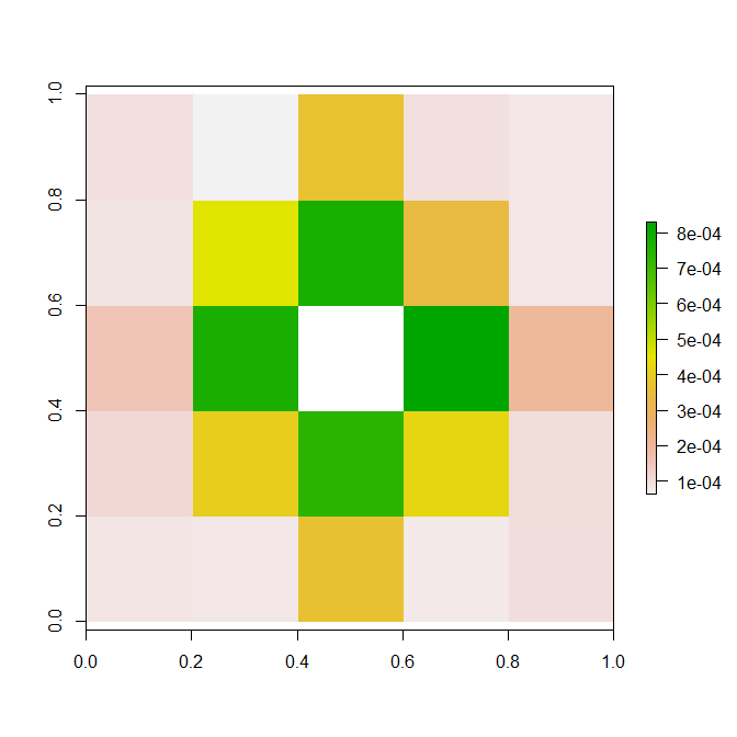
I thought it was interesting how the importance chart didn’t show any one individual pixel as being significant. Is there another similar importance chart or metric that can show the importance of a combination of pixels?
So let’s start by breaking up the current monolithic model into discrete chunks. Once we have done this, it will be easier for us to add new features (which I will do in the next blog). I will store the predicted outputs from each model in image format with separate folders for each model.

The R script for creating the individual models is primarily recycled from my past blogs. Since images contain integer values for pixel brightness, one may argue that storing the predicted values as images loses some of the information content, but the rounding of floating point values to integer values only affects the precision by a maximum of 0.2%, and the noise in the predicted values is an order of magnitude greater than that. If you want that fractional extra predictive power, then I leave it to you to adapt the script to write the floating point predictions into a data.table.
Linear Transformation
The linear transformation model was developed here, and just involves a linear transformation, then constraining the output to be in the [0, 1] range.

# libraries
if (!require("pacman")) install.packages("pacman")
pacman::p_load(png)

dirtyFolder = "C:\\Users\\Colin\\dropbox\\Kaggle\\Denoising Dirty Documents\\data\\train"

# predict using linear transformation
outModel1 = "C:\\Users\\Colin\\dropbox\\Kaggle\\Denoising Dirty Documents\\stacking\\model1"
filenames = list.files(dirtyFolder)
for (f in filenames)
{
print(f)
imgX = readPNG(file.path(dirtyFolder, f))

# turn the images into vectors
x = matrix(imgX, nrow(imgX) * ncol(imgX), 1)

# linear transformation
yHat = -0.126655 + 1.360662 * x

# constrain the range to be in [0, 1]
yHat = sapply(yHat, function(x) max(min(x, 1),0))

# turn the vector into an image
imgYHat = matrix(yHat, nrow(imgX), ncol(imgX))

# save the predicted value
writePNG(imgYHat, file.path(outModel1, f))
}
Thresholding
The thresholding model was developed here, and involves a combination of adaptive thresholding processes, each with different sizes of localisation ranges, plus a global thresholding process. But this time we will use xgboost instead of gbm.

# libraries
if (!require("pacman")) install.packages("pacman")
pacman::p_load(png, data.table, xgboost)

if (!require("EBImage"))
{
source("http://bioconductor.org/biocLite.R")
biocLite("EBImage")
}

# a function to do k-means thresholding
kmeansThreshold = function(img)
{
# fit 3 clusters
v = img2vec(img)
km.mod = kmeans(v, 3)
# allow for the random ordering of the clusters
oc = order(km.mod$centers)
# the higher threshold is the halfway point between the top of the middle cluster and the bottom of the highest cluster
hiThresh = 0.5 * (max(v[km.mod$cluster == oc[2]]) + min(v[km.mod$cluster == oc[3]]))

# using upper threshold
imgHi = v
imgHi[imgHi <= hiThresh] = 0 imgHi[imgHi > hiThresh] = 1

return (imgHi)
}

# a function that applies adaptive thresholding
adaptiveThresholding = function(img)
{
img.eb <- Image(t(img))
img.thresholded.3 = thresh(img.eb, 3, 3)
img.thresholded.5 = thresh(img.eb, 5, 5)
img.thresholded.7 = thresh(img.eb, 7, 7)
img.thresholded.9 = thresh(img.eb, 9, 9)
img.thresholded.11 = thresh(img.eb, 11, 11)
img.kmThresh = kmeansThreshold(img)

# combine the adaptive thresholding
ttt.1 = cbind(img2vec(Image2Mat(img.thresholded.3)), img2vec(Image2Mat(img.thresholded.5)), img2vec(Image2Mat(img.thresholded.7)), img2vec(Image2Mat(img.thresholded.9)), img2vec(Image2Mat(img.thresholded.11)), img2vec(kmeansThreshold(img)))
ttt.2 = apply(ttt.1, 1, max)
ttt.3 = matrix(ttt.2, nrow(img), ncol(img))
return (ttt.3)
}

# a function to turn a matrix image into a vector
img2vec = function(img)
{
return (matrix(img, nrow(img) * ncol(img), 1))
}

# a function to convert an Image into a matrix
Image2Mat = function(Img)
{
m1 = t(matrix(Img, nrow(Img), ncol(Img)))
return(m1)
}

dirtyFolder = "C:\\Users\\Colin\\dropbox\\Kaggle\\Denoising Dirty Documents\\data\\train"
cleanFolder = "C:\\Users\\Colin\\dropbox\\Kaggle\\Denoising Dirty Documents\\data\\train_cleaned"
outPath = "C:\\Users\\Colin\\dropbox\\Kaggle\\Denoising Dirty Documents\\stacking\\model2.csv"
filenames = list.files(dirtyFolder)
for (f in filenames)
{
print(f)
imgX = readPNG(file.path(dirtyFolder, f))
imgY = readPNG(file.path(cleanFolder, f))

# turn the images into vectors
x = img2vec(imgX)
y = img2vec(imgY)

# threshold the image
x2 = kmeansThreshold(imgX)

# adaptive thresholding
x3 = img2vec(adaptiveThresholding(imgX))

dat = data.table(cbind(y, x, x2, x3))
setnames(dat,c("y", "raw", "thresholded", "adaptive"))
write.table(dat, file=outPath, append=(f != filenames[1]), sep=",", row.names=FALSE, col.names=(f == filenames[1]), quote=FALSE)
}

# read in the full data table
dat = read.csv(outPath)

# fit an xgboost model to a subset of the data
set.seed(1)
rows = sample(nrow(dat), 2000000)
dat[is.na(dat)] = 0
dtrain <- xgb.DMatrix(as.matrix(dat[rows,-1]), label = as.matrix(dat[rows,1]))
# do cross validation first
xgb.tab = xgb.cv(data = dtrain, nthread = 8, eval_metric = "rmse", nrounds = 1000, early.stop.round = 50, nfold = 5, print.every.n = 10)
# what is the best number of rounds?
min.error.idx = which.min(xgb.tab[, test.rmse.mean])
# now fit an xgboost model
xgb.mod = xgboost(data = dtrain, nthread = 8, eval_metric = "rmse", nrounds = min.error.idx, print.every.n = 10)

# get the predicted result for each image
outModel2 = "C:\\Users\\Colin\\dropbox\\Kaggle\\Denoising Dirty Documents\\stacking\\model2"
for (f in filenames)
{
print(f)
imgX = readPNG(file.path(dirtyFolder, f))

# turn the images into vectors
x = img2vec(imgX)

# threshold the image
x2 = kmeansThreshold(imgX)

# adaptive thresholding
x3 = img2vec(adaptiveThresholding(imgX))

dat = data.table(cbind(x, x2, x3))
setnames(dat,c("raw", "thresholded", "adaptive"))

# predicted values
yHat = predict(xgb.mod, newdata=as.matrix(dat))

# constrain the range to be in [0, 1]
yHat = sapply(yHat, function(x) max(min(x, 1),0))

# turn the vector into an image
imgYHat = matrix(yHat, nrow(imgX), ncol(imgX))

# save the predicted value
writePNG(imgYHat, file.path(outModel2, f))
}
Edges
The edge model was developed here, and involves a combination of canny edge detection and image morphology.

# libraries
if (!require("pacman")) install.packages("pacman")
pacman::p_load(png, data.table, xgboost, biOps)

# a function to do canny edge detector
cannyEdges = function(img)
{
img.biOps = imagedata(img * 255)
img.canny = imgCanny(img.biOps, 0.7)
return (matrix(img.canny / 255, nrow(img), ncol(img)))
}

# a function combining canny edge detector with morphology
cannyDilated1 = function(img)
{
img.biOps = imagedata(img * 255)
img.canny = imgCanny(img.biOps, 0.7)
# do some morphology on the edges to fill the gaps between them
mat <- matrix (0, 3, 3)
mask <- imagedata (mat, "grey", 3, 3)
img.dilation = imgBinaryDilation(img.canny, mask)
img.erosion = imgBinaryErosion(img.dilation, mask)
return(matrix(img.erosion / 255, nrow(img), ncol(img)))
}

# a function combining canny edge detector with morphology
cannyDilated2 = function(img)
{
img.biOps = imagedata(img * 255)
img.canny = imgCanny(img.biOps, 0.7)
# do some morphology on the edges to fill the gaps between them
mat <- matrix (0, 3, 3)
mask <- imagedata (mat, "grey", 3, 3)
img.dilation = imgBinaryDilation(img.canny, mask)
img.erosion = imgBinaryErosion(img.dilation, mask)
img.erosion.2 = imgBinaryErosion(img.erosion, mask)
img.dilation.2 = imgBinaryDilation(img.erosion.2, mask)
return(matrix(img.dilation.2 / 255, nrow(img), ncol(img)))
}

# a function to turn a matrix image into a vector
img2vec = function(img)
{
return (matrix(img, nrow(img) * ncol(img), 1))
}

dirtyFolder = "C:\\Users\\Colin\\dropbox\\Kaggle\\Denoising Dirty Documents\\data\\train"
cleanFolder = "C:\\Users\\Colin\\dropbox\\Kaggle\\Denoising Dirty Documents\\data\\train_cleaned"
outPath = "C:\\Users\\Colin\\dropbox\\Kaggle\\Denoising Dirty Documents\\stacking\\model3.csv"
filenames = list.files(dirtyFolder)
for (f in filenames)
{
print(f)
imgX = readPNG(file.path(dirtyFolder, f))
imgY = readPNG(file.path(cleanFolder, f))

# turn the images into vectors
x = img2vec(imgX)
y = img2vec(imgY)

# canny edge detector and related features
x4 = img2vec(cannyEdges(imgX))
x5 = img2vec(cannyDilated1(imgX))
x6 = img2vec(cannyDilated2(imgX))

dat = data.table(cbind(y, x, x4, x5, x6))
setnames(dat,c("y", "raw", "canny", "cannyDilated1", "cannyDilated2"))
write.table(dat, file=outPath, append=(f != filenames[1]), sep=",", row.names=FALSE, col.names=(f == filenames[1]), quote=FALSE)
}

# read in the full data table
dat = read.csv(outPath)

# fit an xgboost model to a subset of the data
set.seed(1)
rows = sample(nrow(dat), 2000000)
dat[is.na(dat)] = 0
dtrain <- xgb.DMatrix(as.matrix(dat[rows,-1]), label = as.matrix(dat[rows,1]))
# do cross validation first
xgb.tab = xgb.cv(data = dtrain, nthread = 8, eval_metric = "rmse", nrounds = 1000, early.stop.round = 50, nfold = 5, print.every.n = 10)
# what is the best number of rounds?
min.error.idx = which.min(xgb.tab[, test.rmse.mean])
# now fit an xgboost model
xgb.mod = xgboost(data = dtrain, nthread = 8, eval_metric = "rmse", nrounds = min.error.idx, print.every.n = 10)

# get the predicted result for each image
outModel3 = "C:\\Users\\Colin\\dropbox\\Kaggle\\Denoising Dirty Documents\\stacking\\model3"
for (f in filenames)
{
print(f)
imgX = readPNG(file.path(dirtyFolder, f))

# turn the images into vectors
x = img2vec(imgX)

# canny edge detector and related features
x4 = img2vec(cannyEdges(imgX))
x5 = img2vec(cannyDilated1(imgX))
x6 = img2vec(cannyDilated2(imgX))

dat = data.table(cbind(x, x4, x5, x6))
setnames(dat,c("raw", "canny", "cannyDilated1", "cannyDilated2"))

# predicted values
yHat = predict(xgb.mod, newdata=as.matrix(dat))

# constrain the range to be in [0, 1]
yHat = sapply(yHat, function(x) max(min(x, 1),0))

# turn the vector into an image
imgYHat = matrix(yHat, nrow(imgX), ncol(imgX))

# save the predicted value
writePNG(imgYHat, file.path(outModel3, f))
}
Background Removal
The background removal model was developed here, and involves the use of median filters. An xgboost model is used to combine the median filter results.

# libraries
if (!require("pacman")) install.packages("pacman")
pacman::p_load(png, data.table, xgboost)
# a function to do a median filter
median_Filter = function(img, filterWidth)
{
pad = floor(filterWidth / 2)
padded = matrix(NA, nrow(img) + 2 * pad, ncol(img) + 2 * pad)
padded[pad + seq_len(nrow(img)), pad + seq_len(ncol(img))] = img

tab = matrix(NA, nrow(img) * ncol(img), filterWidth ^ 2)
k = 1
for (i in seq_len(filterWidth))
{
for (j in seq_len(filterWidth))
{
tab[,k] = img2vec(padded[i - 1 + seq_len(nrow(img)), j - 1 + seq_len(ncol(img))])
k = k + 1
}
}

filtered = unlist(apply(tab, 1, function(x) median(x, na.rm = TRUE)))
return (matrix(filtered, nrow(img), ncol(img)))
}

# a function that uses median filter to get the background then finds the dark foreground
background_Removal = function(img)
{
w = 5

# the background is found via a median filter
background = median_Filter(img, w)

# the foreground is darker than the background
foreground = img - background
foreground[foreground > 0] = 0
m1 = min(foreground)
m2 = max(foreground)
foreground = (foreground - m1) / (m2 - m1)

return (matrix(foreground, nrow(img), ncol(img)))
}

# a function to turn a matrix image into a vector
img2vec = function(img)
{
return (matrix(img, nrow(img) * ncol(img), 1))
}

dirtyFolder = "C:\\Users\\Colin\\dropbox\\Kaggle\\Denoising Dirty Documents\\data\\train"
cleanFolder = "C:\\Users\\Colin\\dropbox\\Kaggle\\Denoising Dirty Documents\\data\\train_cleaned"
outPath = "C:\\Users\\Colin\\dropbox\\Kaggle\\Denoising Dirty Documents\\stacking\\model4.csv"
filenames = list.files(dirtyFolder)
for (f in filenames)
{
print(f)
imgX = readPNG(file.path(dirtyFolder, f))
imgY = readPNG(file.path(cleanFolder, f))

# turn the images into vectors
x = img2vec(imgX)
y = img2vec(imgY)

# median filter and related features
x7a = img2vec(median_Filter(imgX, 5))
x7b = img2vec(median_Filter(imgX, 11))
x7c = img2vec(median_Filter(imgX, 17))
x8 = img2vec(background_Removal(imgX))

dat = data.table(cbind(y, x, x7a, x7b, x7c, x8))
setnames(dat,c("y", "raw", "median5", "median11", "median17", "background"))
write.table(dat, file=outPath, append=(f != filenames[1]), sep=",", row.names=FALSE, col.names=(f == filenames[1]), quote=FALSE)
}

# read in the full data table
dat = read.csv(outPath)

# fit an xgboost model to a subset of the data
set.seed(1)
rows = sample(nrow(dat), 2000000)
dat[is.na(dat)] = 0
dtrain <- xgb.DMatrix(as.matrix(dat[rows,-1]), label = as.matrix(dat[rows,1]))
# do cross validation first
xgb.tab = xgb.cv(data = dtrain, nthread = 8, eval_metric = "rmse", nrounds = 1000, early.stop.round = 50, nfold = 5, print.every.n = 10)
# what is the best number of rounds?
min.error.idx = which.min(xgb.tab[, test.rmse.mean])
# now fit an xgboost model
xgb.mod = xgboost(data = dtrain, nthread = 8, eval_metric = "rmse", nrounds = min.error.idx, print.every.n = 10)

# get the predicted result for each image
outModel4 = "C:\\Users\\Colin\\dropbox\\Kaggle\\Denoising Dirty Documents\\stacking\\model4"
for (f in filenames)
{
print(f)
imgX = readPNG(file.path(dirtyFolder, f))

# turn the images into vectors
x = img2vec(imgX)

# median filter and related features
x7a = img2vec(median_Filter(imgX, 5))
x7b = img2vec(median_Filter(imgX, 11))
x7c = img2vec(median_Filter(imgX, 17))
x8 = img2vec(background_Removal(imgX))

dat = data.table(cbind(x, x7a, x7b, x7c, x8))
setnames(dat,c("raw", "median5", "median11", "median17", "background"))

# predicted values
yHat = predict(xgb.mod, newdata=as.matrix(dat))

# constrain the range to be in [0, 1]
yHat = sapply(yHat, function(x) max(min(x, 1),0))

# turn the vector into an image
imgYHat = matrix(yHat, nrow(imgX), ncol(imgX))

# save the predicted value
writePNG(imgYHat, file.path(outModel4, f))
}
Nearby Pixels
The spacial model was developed here, and involves the use of a sliding window and xgboost.
# libraries
if (!require("pacman")) install.packages("pacman")
pacman::p_load(png, data.table, xgboost)

# a function that groups together the pixels contained within a sliding window around each pixel of interest
proximalPixels = function(img)
{
 pad = 2
 width = 2 * pad + 1
 padded = matrix(median(img), nrow(img) + 2 * pad, ncol(img) + 2 * pad)
 padded[pad + seq_len(nrow(img)), pad + seq_len(ncol(img))] = img

 tab = matrix(1, nrow(img) * ncol(img), width ^ 2)
 k = 1
 for (i in seq_len(width))
 {
 for (j in seq_len(width))
 {
 tab[,k] = img2vec(padded[i - 1 + seq_len(nrow(img)), j - 1 + seq_len(ncol(img))])
 k = k + 1
 }
 }

 return (tab)
}

# a function to turn a matrix image into a vector
img2vec = function(img)
{
 return (matrix(img, nrow(img) * ncol(img), 1))
}

dirtyFolder = "C:\\Users\\Colin\\dropbox\\Kaggle\\Denoising Dirty Documents\\data\\train"
cleanFolder = "C:\\Users\\Colin\\dropbox\\Kaggle\\Denoising Dirty Documents\\data\\train_cleaned"
outPath = "C:\\Users\\Colin\\dropbox\\Kaggle\\Denoising Dirty Documents\\stacking\\model5.csv"
filenames = list.files(dirtyFolder)
for (f in filenames)
{
 print(f)
 imgX = readPNG(file.path(dirtyFolder, f))
 imgY = readPNG(file.path(cleanFolder, f))

 # turn the images into vectors
 #x = img2vec(imgX)
 y = img2vec(imgY)

 # surrounding pixels
 x9 = proximalPixels(imgX)

 dat = data.table(cbind(y, x9))
 setnames(dat,append("y", paste("x", 1:25, sep="")))
 write.table(dat, file=outPath, append=(f != filenames[1]), sep=",", row.names=FALSE, col.names=(f == filenames[1]), quote=FALSE)
}

# read in the full data table
dat = read.csv(outPath)

# fit an xgboost model to a subset of the data
set.seed(1)
rows = sample(nrow(dat), 2000000)
dat[is.na(dat)] = 0
dtrain <- xgb.DMatrix(as.matrix(dat[rows,-1]), label = as.matrix(dat[rows,1]))
# do cross validation first
xgb.tab = xgb.cv(data = dtrain, nthread = 8, eval_metric = "rmse", nrounds = 1000, early.stop.round = 50, nfold = 5, print.every.n = 10)
# what is the best number of rounds?
min.error.idx = which.min(xgb.tab[, test.rmse.mean])
# now fit an xgboost model
xgb.mod = xgboost(data = dtrain, nthread = 8, eval_metric = "rmse", nrounds = min.error.idx, print.every.n = 10)


# get the predicted result for each image
outModel5 = "C:\\Users\\Colin\\dropbox\\Kaggle\\Denoising Dirty Documents\\stacking\\model5"
for (f in filenames)
{
 print(f)
 imgX = readPNG(file.path(dirtyFolder, f))

 # turn the images into vectors
 #x = img2vec(imgX)

 # surrounding pixels
 x9 = proximalPixels(imgX)

 dat = data.table(x9)
 setnames(dat,paste("x", 1:25, sep=""))

 # predicted values
 yHat = predict(xgb.mod, newdata=as.matrix(dat))

 # constrain the range to be in [0, 1]
 yHat = sapply(yHat, function(x) max(min(x, 1),0))

 # turn the vector into an image
 imgYHat = matrix(yHat, nrow(imgX), ncol(imgX))

 # save the predicted value
 writePNG(imgYHat, file.path(outModel5, f))
}
Combining the Individual Models
There are many ways that the predictions of the models could be ensembled together. I have used an xgboost model because I want to allow for the complexity of the problem that is being solved.
# libraries
if (!require("pacman")) install.packages("pacman")
pacman::p_load(png, data.table, xgboost)

# a function to turn a matrix image into a vector
img2vec = function(img)
{
 return (matrix(img, nrow(img) * ncol(img), 1))
}

inPath1 = "C:\\Users\\Colin\\dropbox\\Kaggle\\Denoising Dirty Documents\\stacking\\model1"
inPath2 = "C:\\Users\\Colin\\dropbox\\Kaggle\\Denoising Dirty Documents\\stacking\\model2"
inPath3 = "C:\\Users\\Colin\\dropbox\\Kaggle\\Denoising Dirty Documents\\stacking\\model3"
inPath4 = "C:\\Users\\Colin\\dropbox\\Kaggle\\Denoising Dirty Documents\\stacking\\model4"
inPath5 = "C:\\Users\\Colin\\dropbox\\Kaggle\\Denoising Dirty Documents\\stacking\\model5"

cleanFolder = "C:\\Users\\Colin\\dropbox\\Kaggle\\Denoising Dirty Documents\\data\\train_cleaned"
outPath = "C:\\Users\\Colin\\dropbox\\Kaggle\\Denoising Dirty Documents\\stacking\\stacking.csv"

filenames = list.files(inPath1)
for (f in filenames)
{
 print(f)
 imgX1 = readPNG(file.path(inPath1, f))
 imgX2 = readPNG(file.path(inPath2, f))
 imgX3 = readPNG(file.path(inPath3, f))
 imgX4 = readPNG(file.path(inPath4, f))
 imgX5 = readPNG(file.path(inPath5, f))
 imgY = readPNG(file.path(cleanFolder, f))

 # turn the images into vectors
 #x = img2vec(imgX)
 y = img2vec(imgY)

 # contributing models
 x1 = img2vec(imgX1)
 x2 = img2vec(imgX2)
 x3 = img2vec(imgX3)
 x4 = img2vec(imgX4)
 x5 = img2vec(imgX5)

 dat = data.table(cbind(y, x1, x2, x3, x4, x5))
 setnames(dat,c("y", "linear", "thresholding", "edges", "backgroundRemoval", "proximal"))
 write.table(dat, file=outPath, append=(f != filenames[1]), sep=",", row.names=FALSE, col.names=(f == filenames[1]), quote=FALSE)
}

# read in the full data table
dat = read.csv(outPath)

# fit an xgboost model to a subset of the data
set.seed(1)
rows = sample(nrow(dat), 5000000)
dat[is.na(dat)] = 0
dtrain <- xgb.DMatrix(as.matrix(dat[rows,-1]), label = as.matrix(dat[rows,1]))
# do cross validation first
xgb.tab = xgb.cv(data = dtrain, nthread = 8, eval_metric = "rmse", nrounds = 1000, early.stop.round = 50, nfold = 5, print.every.n = 10)
# what is the best number of rounds?
min.error.idx = which.min(xgb.tab[, test.rmse.mean])
# now fit an xgboost model
xgb.mod = xgboost(data = dtrain, nthread = 8, eval_metric = "rmse", nrounds = min.error.idx, print.every.n = 10)

# get the trained model
model = xgb.dump(xgb.mod, with.stats=TRUE)
# get the feature real names
names = names(dat)[-1]
# compute feature importance matrix
importance_matrix = xgb.importance(names, model=xgb.mod)
# plot the variable importance
gp = xgb.plot.importance(importance_matrix)
print(gp)

# get the predicted result for each image
outModel = "C:\\Users\\Colin\\dropbox\\Kaggle\\Denoising Dirty Documents\\stacking\\stacked"
for (f in filenames)
{
 print(f)
 imgX1 = readPNG(file.path(inPath1, f))
 imgX2 = readPNG(file.path(inPath2, f))
 imgX3 = readPNG(file.path(inPath3, f))
 imgX4 = readPNG(file.path(inPath4, f))
 imgX5 = readPNG(file.path(inPath5, f))

 # contributing models
 x1 = img2vec(imgX1)
 x2 = img2vec(imgX2)
 x3 = img2vec(imgX3)
 x4 = img2vec(imgX4)
 x5 = img2vec(imgX5)

 dat = data.table(cbind(x1, x2, x3, x4, x5))
 setnames(dat,c("linear", "thresholding", "edges", "backgroundRemoval", "proximal"))

 # predicted values
 yHat = predict(xgb.mod, newdata=as.matrix(dat))

 # constrain the range to be in [0, 1]
 yHat = sapply(yHat, function(x) max(min(x, 1),0))

 # turn the vector into an image
 imgYHat = matrix(yHat, nrow(imgX1), ncol(imgX1))

 # save the predicted value
 writePNG(imgYHat, file.path(outModel, f))
}

The graph above answers Bobby’s question – when considered together, the nearby pixels provide most of the additional predictive power beyond that of the raw pixel brightness. It seems that the key to separating dark text from noise is to consider how the pixel fits into the local region within the image.
Now that we have set up a stacking model structure, we can recommence the process of adding more image processing and features to the model. And that’s what the next blog will do…

Great post Colin! Answers my question perfectly :).
LikeLiked by 1 person
Hi Bobby. I was actually surprised by the feature importance result, because it basically says that the other model inputs are almost worthless, and I don’t believe that. But one of the top Kaggle competitors told me that xgboost’s importance measures can be off sometimes. So it would be interesting to rerun this stacking using a gbm model to see what importance measure it says.
LikeLike
Pingback: Denoising Dirty Documents: Part 8 | Keeping Up With The Latest Techniques